When are two words better than one? Informative n-grams for Text Sentiment Classification

Text classification is a fundamental problem type in NLP and also serves as a common benchmark task in evaluating representations of text for machine learning. In this post, I’ll use the Large Movie Review Dataset from Maas et al. (2011). This dataset provides 25,000 movie reviews from IMDb for the benchmark task of classifying reviews as either positive (user rating 7-10) or negative (user rating 1-4). This task is known as sentiment analysis but the techniques are applicable to other text classification problems like spam filtering, topic classification and language detection.

A simple and useful way to represent text for classification is the bag of words. Each text is represented as a vector with length equal to the vocabulary size, where the value indicates the number of times that word occurs in the text.

An obvious drawback to this method is it completely ignores any information about word order. It’s therefore unable to capture more complex aspects of meaning encoded in the relationships between words and phrases, or to distinguish between different senses of a word.

In this post, we’ll mitigate this problem by including highly informative bigrams and trigrams in addition to individual words. Since the number of unique bigrams and trigrams is very large, and most of them are rare and indicate a sentiment polarity roughly consistent with that of their component words, we don’t want to include them all in the model and end up with tens of thousands of uninformative features. Instead we’ll select only the bigrams and trigrams with estimated polarity that is significantly different from what would be expected based on the individual words.

Data Preparation

I tokenized the texts into words, removing any HTML tags. I also separated the training data into a training (70%) and validation (30%) set. The resulting training set consists of 17,500 movie reviews, evenly split between positive and negative. 90% of the review lengths are between 75 and 698 words. Our movie review samples then look something like this (feature generation will ignore capitalization and drop punctuation tokens):

['This', 'is', 'not', 'the', 'typical', 'Mel', 'Brooks', 'film', '.', 'It', 'was', 'much', 'less', 'slapstick', ...]

Positive and Negative Sentiment Words

First, let’s check which words have the strongest sentiment polarity signals. Our numerical measure of polarity will be the log of the ratio of the word’s frequency in positive reviews versus negative reviews. Restricting to words with frequency at least 1 in 10,000, the most positive and negative words are:

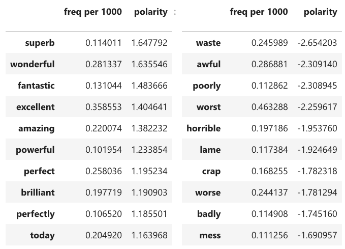
That makes sense, although I was surprised that today is so much more common in positive reviews.

Unexpectedly Positive and Negative n-Grams

There are 78,295 unique words, 125,004 unique bigrams, and 495,856 unique trigrams in the training set. Since most of these are uninformative, we want to select the most relevant bigrams and trigrams to augment the bag-of-words feature set.

I used a linear model to estimate the expected polarity of each n-gram based on its component words. I trained separate models for bigrams and trigrams. Using all n-grams that appeared at least once in every 50,000 tokens, I trained a linear model with coefficients for the polarities of the most polar word, least polar word, and intermediate polarity word (for the trigram model):

CoefficientsBigram ModelTrigram Model
Least polar0.6250.188
Intermediate0.733
Most polar1.1181.238

It is mostly the most polar word within an n-gram that defines the polarity of the n-gram overall, although all words matter to some extent.

We can then identify bigrams and trigrams that are more positive or more negative than expected and select only those to use as model features.

Plotting trigram polarity against expected polarity based on word-level linear model. Dot size indicates trigram frequency. Trigrams with residual polarity greater than 1 or less than -1 are highlighted in blue/red.

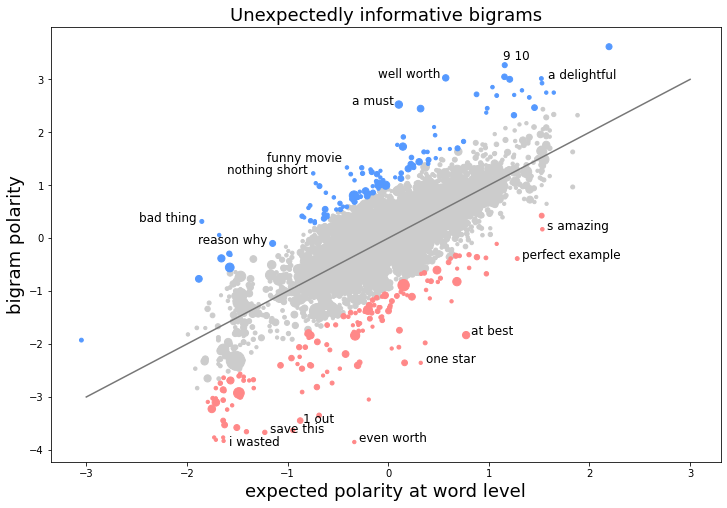
Positive bigrams made out of negative words include bad thing (as in, the one bad thing about this good movie) and “reason why”. Bigrams that are expected to be positive but turn out to be even more so include 9/10 and a delightful. Negative bigrams made out of positive words include at best and one star. Bigrams that are expected to be negative but turn out to be even more so include I wasted and save this.

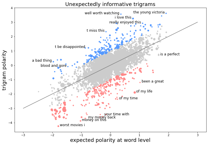
The same analysis with trigrams turns up some characteristically multi-word sentiment indicators like (you won’)t be disappointed and (would have) been a great, but also some that appear to be movie-specific (blood and gore, the young victoria) that we might not expect to generalize.

Feature Selection

The next step is to select a subset of the ~700,000 features to include in the model. I decided to select bigrams and trigrams using a minimum cutoff for frequency and polarity, and then fill with the top words (ranked by frequency with a small adjustment for polarity to boost high-polarity words near the frequency cutoff) up to the desired total number of features. The cutoff levels are hyperparameters that I set by choosing values that give good predictions on the validation set. I also consider models that drop stopwords (common, nonspecific words like the, for, and).

Logistic Regression Model

scikitlearn’s implementation of logistic regression is a basic but effective technique for binary classification. Below are my top results on the validation set with different settings for feature generation:

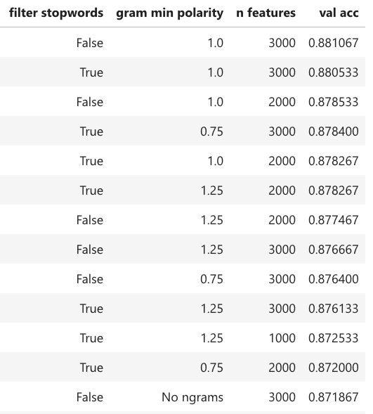
The best results are obtained with no stopword filtering, minimum n-gram polarity of 1 (log ratio units) and 3000 total features. Adding n-grams to the model improves the accuracy by almost 1 percentage point compared to the pure bag-of-words model.

Training with Keras

To evaluate how the augmented bag of words features perform with different model types, I also trained a neural net model using Keras. I used a feed-forward fully connected network with two hidden layers, ReLu activation function and binary cross-entropy loss. I set the training to stop early when the validation accuracy no longer increased with additional epochs. This training takes a couple of minutes on my laptop’s CPU.

Results

Although the neural net model performed better on validation, it was slightly worse on test (maybe using the validation results to choose the stopping epoch slightly biased the validation accuracy upward). Overall, we achieve 88% accuracy which is comparable to benchmark results using methods based on bag of words representations. For comparison, 93% accuracy has been reported on this dataset using BERT, a state-of-the-art sequence-based text representation trained on very large text corpora.

Logistic Regression0.8799
Feed-forward NN0.8785
Keras Tutorial (Vector embedding + Convolutional NN)0.8650
Maas et al. (2011) Baseline (Bag of Words SVM)0.8780
Maas et al. (2011) Full (Bag of Words + Semantic/Sentiment Vector SVM)0.8889
BERT (Sanh et al., 2019)0.9346

Discussion

One might think it would be easier to get over 90% accuracy on this task as the texts are relatively clean and relevant and the training set is large. What kinds of language are confusing the model? Looking at some misclassified texts we can see some patterns. Often, positive-sentiment or negative-sentiment language occurs but refers to something other than the movie. For instance, one review praised a film for its willingness to portray negative aspects of its historical protagonist. One negative review even contained the phrase “extremely well written” in reference to another user’s critical comments about the film. Without the ability to bind comments to topics, we can only identify reviews with a preponderance of positive or negative comments, but not the specific entity that is being praised or criticized.

Another tendency of the reviews is to flip back and forth between positive and negative comments, ending with something like “Overall, it is fun to watch.” Expressions like Overall or All in all or In the end cue the reader to interpret the following comment as a global assessment of the film whereas opposite-polarity comments are specific to particular aspects that don’t make or break it, but our model can’t learn to condition the importance of one phrase on its position in the discourse relative to another.

Other times, reviewers expressed the idea of the movie being good or bad, but not actually making that assertion, e.g. people said this was a great movie. Our model isn’t able to detect the contextual cues that distinguish direct statements from various types of indirect speech, quotations, sarcasm, rhetorical questions, and the like.

Overall, our n-gram selection technique efficiently upgrades the bag-of-words model to a bag-of-words-and-phrases model without significantly increasing the size of the model, as would be necessary for a full bigram or trigram model. We achieve decent results with either logistic regression or feed-forward NN by detecting positive or negative linguistic elements. However, the performance of our model is limited by its lack of any level of language understanding that could reliably distinguish between positive/negative sentiment statements that make assertions about the main topic and those that do not.

Code

View the Python code used for this post at: https://github.com/lucasmchang/text_classification/blob/main/movie_reviews_sentiment.ipynb

A Very Brief History of the Chinese Language

I very much enjoyed Hongyuan Dong’s A History of the Chinese Language, which packs about as much information as possible into 200 pages while being about as readable as you can hope for. Here is 3000+ years of linguistic history further compressed into about six screens:

1. The Sino-Tibetan Language Family

Chinese is in the Sino-Tibetan language family. Other languages in the family include the Tibetan languages, Burmese, and other less well known languages scattered around the Himalayas and Southeast Asia.

The Chinese languages have no close cousins, as the other groups of Sino-Tibetan languages diverged many thousands of years ago and are not obviously similar.

Some linguists think the Tai-Kadai (including Thai and Lao) and the Hmong-Mien languages of southern China and Southeast Asia are related, but the consensus view is that the similarities are due to millennia of contact, not a common origin. Vietnamese is quite similar to Chinese on the surface, but this is certainly due to contact.

2. The Varieties of Chinese

Much ink has been spent on the question of whether the varieties of Chinese are “languages” or “dialects”. In China they are generally called 方言 “local speech.” 

The regional varieties are classified in seven main groups. The Mandarin group includes the standard language, based on Beijing speech, and a vast swath of dialects in northern, central, and southwestern China. The other groups are mostly spoken in the southeast and include Cantonese, Shanghainese, Taiwanese Hokkien, and Hakka among others.

The varieties are not just different accents; they are different enough that speakers either cannot understand each other at all or only with difficulty, comparable to speakers of Spanish, Portuguese, French, and Italian. The varieties are, however, tied together by a shared formal written form (previously Classical, now Mandarin), and of course the standard language is increasingly present everywhere.

Non-Chinese languages are also native to frontier areas of Northern, Southern, and Western China, isolated pockets in Southern China, and indigenous Taiwanese.

3. Old Chinese: Confucius’ Language

Old Chinese covers the period from the earliest inscriptions in the 1000s BC through the Han Dynasty in the third century. There is an extensive written corpus including the Confucian and Daoist classics, and in fact until the 20th century, Classical or Literary Chinese based on this form of the language was the main written standard. 

Although we have many Old Chinese texts, it is still difficult to reconstruct the pronunciation because Old Chinese was never recorded in a phonetic script. The main sources of information on the pronunciation are:

1. The Classic of Poetry 詩經, a collection of poems with a clear rhyming structure. We can assume that if two characters rhyme in these poems, then they would have rhymed in spoken Old Chinese.

2. Chinese characters themselves often contain a component that is a phonetic “hint”, and we can assume similar pronunciations for sets of characters with the same hint (e.g. the element 皮 indicates that 疲被陂 should have been pronounced similarly).

3. Extrapolating backward from Middle Chinese pronunciation, which we know a little more about.

Linguists have done this and reconstructed a pronunciation that looks quite unfamiliar to us these days. It lacks tones and it contains many consonant clusters unlike anything in the modern Chinese languages. For instance 兼葭蒼蒼 白露為霜 is jiān jiā cāng cāng bái lù wéi shuāng in Mandarin, but is reconstructed as something like kem kra tsang tsang brak praks gwraj srang. Of course, Old Chinese was spoken for over a thousand years in a vast empire, so the reconstructed pronunciation only represents its general structure and not any specific real person’s speech.

As for the grammar of Old Chinese, its syntax is actually quite different from modern Chinese, but neither language has much inflection or complex morphology. There might have been more inflection in archaic forms of Old Chinese, vestiges of which survive today in the form of characters that are used for two distinct but related words (e.g. 傳 is used for both chuán “to transmit” and zhuàn “a record”) but it is difficult to reconstruct that sort of thing from non-phonetic written records.

4. Middle Chinese: Li Bai’s Language

Middle Chinese covers the period from the fall of the Han to the Song dynasty in the 13th century. This period encompasses the Tang dynasty poets such as Li Bai, who are still widely read.

During the Middle Chinese period, Chinese scholars started to write about how their language was pronounced. With dictionaries and tabulations such as the Qieyun (切韻) , we have clear indications about which characters were pronounced the same in the prestige dialect, as well as somewhat less clear indications about their phonetic realization.

The dictionaries and tables give us most of our knowledge about the abstract phonological structure of Middle Chinese, but the precise phonetic details are mostly reconstructed by comparing the present-day dialectal forms. To a lesser extent, we can also learn about the pronunciation by examining the forms of loanwords from Sanskrit into Chinese and from Chinese into Japanese, Korean, and Vietnamese.

The sounds of Li Bai’s language are recognizably Chinese, though no longer intelligible to a Mandarin speaker. Like Mandarin, it had four tones (although they don’t match up one-to-one with the tones of Mandarin) and the syllable structure was similar, though several mergers and splits separate it from modern forms in the details.

By this time, the vernacular language had diverged from the classical language still used in most writing.

5. Vernacular Writing and Early Mandarin

Although most people wrote in Classical Chinese, we can see new developments in the grammar and vocabulary of the language in two ways:

1. Vernacular writing such as folk songs, plays and novels

2. New constructions popping up in otherwise classical documents

Using these two methods, many of the grammatical and lexical differences between contemporary Mandarin and Classical Chinese can be traced back several centuries. We can assume that these changes accumulated gradually in the spoken vernaculars.

By the start of the Yuan dynasty in the 13th century, the spoken language of northern China was recognizable as an early form of Mandarin.

6. Modernity and Standardization

Around the end of the Qing dynasty at the start of the 20th century, linguistic reform became associated with modernity. Intellectuals spurred a change from literary Chinese to writing in vernacular Mandarin, and this was made official by the Republic of China government. Both the Mainland and Taiwan governments established official standard spoken languages based on Beijing Mandarin. Many words for modern scientific, political, and economic concepts were either coined using Chinese word roots to translate foreign words or borrowed from Japanese terms that had themselves been coined using Chinese word roots.

7. Chinese Characters

Most of what you read about Chinese characters is half-truths, this included.

The oldest known Chinese characters are inscribed on the “oracle bones” of the 2nd millennium BCE. These are already Chinese characters proper, not merely pictographic proto-writing. Therefore, there must have been earlier stages that have not been preserved.

Character shapes recognizable as early forms of those in use today were first standardized in the Qin dynasty (3rd century BCE).

Characters come in several types:

1. A few characters are pictograms. 

2. A few characters are pictograms with added marks to indicate abstract meaning.

3. A few characters are compounds of pictograms.

4a. Most characters are compounds of a phonetic element and a semantic element.

4b. Some characters have a semantic hint, but the other element is not purely phonetic.

5. A few characters are re-purposed or variant forms of other characters.

8. In Conclusion

In English and many other world languages, most of what we think of as the forces shaping the modern forms are thought of as coming from outside: Latin, Greek, French, Christianity, the colonial empires and globalization. Chinese linguistic history is much more inward-facing and tends to draw attention to deeper time scales. In both cases, today’s linguistic forms are deeply marked by the traces of linguistic history as well as cultural traditions regarding literature and identity.

The Great Vowel Shift, or why English vowel spellings confuse the world

Why is there such a mismatch between the sounds represented by the vowel letters in English versus virtually every other language that uses the Latin alphabet? For instance, “oo” makes the /uː/ sound that rightfully belongs to the letter U. “ee” and “ea” make the /i:/ sound that is normally written I, and “a” can either be the expected /ɑ/ or the unusual /eɪ/. 

Contrast this with a language like Spanish, where the symbols A E I O U represent the sounds “ah” “eh” “ee” “oh” “oo,” with the letters and their values inherited from Latin. Other European languages have more complex vowel inventories, but at least the most fundamental values of the vowel letters — sometimes called the “continental” values — tend to be preserved.

Why don’t we spell “eye” ai, “food” fuud, or “treaty” triti? The explanation depends on something called the Great Vowel Shift. Continue reading The Great Vowel Shift, or why English vowel spellings confuse the world

Low-Yield Searches: Availability of Information on Wikipedia Affects Tourist Decisions

Two roads diverged in a wood, and I — I looked them up on Wikipedia

Have you ever looked something up on Wikipedia or Google and failed to find much relevant or high-quality content? Every time that happens, it’s a subtle hint to us that the topic isn’t important or interesting. However, this implicit message is often biased, especially against diversity and in favor of the dominant culture and its language and trends.  Continue reading Low-Yield Searches: Availability of Information on Wikipedia Affects Tourist Decisions

Did Homo erectus have language? According to Daniel Everett, they invented it

Review of the book How Language Began: The Story of Humanity’s Greatest Invention:

In grad school, I remember hearing about Daniel Everett as a controversial and somewhat heterodox figure in the world of linguistics, but until now I had never read any of his work.

Everett’s controversial claim is that a lot of the structural and especially syntactic features of human languages that are commonly thought to be universal, and without which language would be unimaginable, are actually not universal and not fundamental at all.

He bases this claim on his observations of the languages spoken in the Brazilian Amazon, especially Pirahã. Continue reading Did Homo erectus have language? According to Daniel Everett, they invented it

The Scots Wikipedia Thing

The Scots Wikipedia thing is changing the way I think about the Internet and minority languages.

What happened?

Earlier this week [originally written August 28, 2020], a viral Reddit post alleged that a single editor — a non-Scots-speaking American — of the Scots-language Wikipedia has flooded the wiki with, essentially, mangled English articles translated into fake Scots, mostly by substituting word-for-word using an English-Scots dictionary. (The user in question seems to have acted in good faith; he started as a child and has apologized). Other non-Scots-speaking editors have also made many low-quality contributions. Apparently, there was never a sufficient community of actual Scots speakers on Wikipedia to keep the poor-quality “Scotched English” in check and fill the wiki with authentic Scots articles. Now the Scots Wikipedia community is stuck with the question of what to do with this fiasco of a Wikipedia: delete it, roll back to an older version, mobilize the Scots-speaking community to fix all the articles? Continue reading The Scots Wikipedia Thing

Reconstructing geographic distance among cities using distributional semantics


Estimated map of the 100 most populous US cities constructed by predicting the distances between them based on their similarity in Word2Vec semantic space. 


The way we use words in language encodes a lot of information about the real-world meaning of those words. Continue reading Reconstructing geographic distance among cities using distributional semantics

What country is the happiest? Interpreting ordinal-scale data


In this post, I model the latent distribution of national happiness using self-report data, and discuss the difficulties involved in ranking countries by “average” happiness.


Often, when studying people’s subjective experiences, data are collected by asking survey participants to report on an ordinal scale how much they agree with a statement or question. Continue reading What country is the happiest? Interpreting ordinal-scale data